26 Oct 2023

Adriana Nicoara
Junior Data Scientist

Multi-Label text classification: Overview and step-by-step tutorial

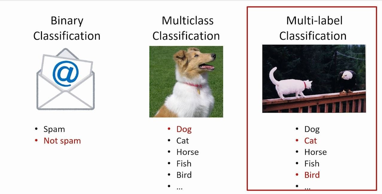
Classification is an AI text analysis technique that automatically labels previously undiscovered text. There are three primary types of classification problems: binary, multiclass and multi-label.

In a binary classification, there can be only two categories (classes) and an item can belong only to one of the two categories. In contrast to binary classification, in a multi-class classification, there can be more than two categories and an item can belong to only one category. In a multi-label classification there are multiple categories and an item can have more than one category.

Image source

In this article we will focus on multi-label classification of text documents.

Machine learning and natural language processing are the key techniques when it comes to text classification, because they enable automated analysis of text, context understanding and adaptability to various domains.

As machine learning problems can be divided into supervised and unsupervised learning, classification represents a major part of supervised problems.

Now let’s take a closer look into each step needed to construct a text classification algorithm.

Dataset

The dataset used in this tutorial is the PubMed MultiLabel Text Classification Dataset MeSH publicly available on Kaggle.

This dataset consists of a large number of research articles which are annotated with their MeSH labels. These labels are organized into a hierarchical structure of classes and subclasses, but for the sake of clarity, we will focus only on the general labels from the root. There is a total of 14 unique labels in the root MeSH classification (A: Anatomy, B: Organism, C: Diseases, etc.) and an article can have more than one label.

import pandas as pd
dataset_path = "dataset/PubMed Multi Label Text Classification Dataset Processed.csv"
dataframe = pd.read_csv(dataset_path)
dataframe.head(5)

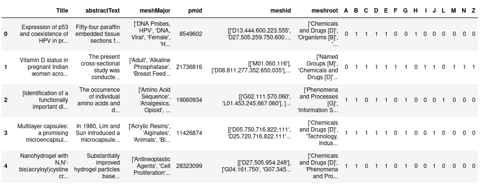
The objective of this tutorial is to assign MeSH labels to unseen articles.

Dataset analysis

Now, let’s explore the dataset by starting with its attributes.

print("Total number of articles: ", dataframe.shape[0])
print("Total number of columns in the dataset: ", dataframe.shape[1])

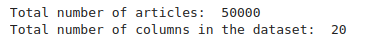
In the dataset there are 50000 articles available for training and testing. The dataset contains multiple features, represented by columns.

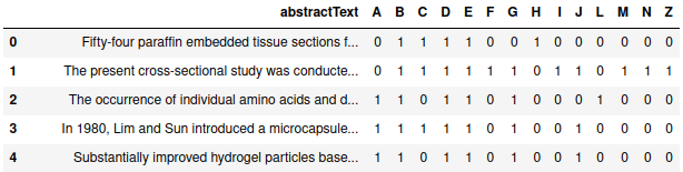
Not all features are relevant for the classification task and we want to predict labels based on the article’s content. Therefore, we will keep only the abstractText, which is the summarization of the article and the columns associated to the 14 labels.

trimmed_dataframe = dataframe.drop(['Title', 'meshMajor', 'pmid', 'meshid','meshroot'], axis = 1)

labels = trimmed_dataframe.iloc[:, 1:].sum()
print("Total labels: ",labels.sum())

rowsums=trimmed_dataframe.iloc[:,1:].sum(axis=1)
no_label_count = 0
for sum in rowsums.values:
    if sum==0:
        no_label_count +=1
print("Total number of articles without label: ", no_label_count)

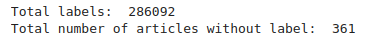
Apparently there are 361 articles without any label, so let’s plot a graph to see more precisely the class distribution.

import matplotlib.pyplot as plt
import seaborn as sns

x=trimmed_dataframe.iloc[:,1:].sum()
plt.figure(figsize=(9,9))
ax= sns.barplot(x=x.index, y=x.values, alpha=0.8)
plt.title("Class count")
plt.ylabel('Number of Occurrences', fontsize=12)
plt.xlabel('Label', fontsize=12)

rects = ax.patches
labels = x.values
for rect, label in zip(rects, labels):
    height = rect.get_height()
    ax.text(rect.get_x() + rect.get_width()/2, height + 5, label, ha='center', va='bottom')

plt.show()

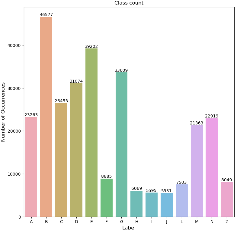
The most popular label is B: Organism. We can clearly see that the dataset is highly imbalanced, the number of articles per label varying a lot. This aspect may negatively impact the performance of the trained model. But for now, let’s move on to the next graph, which represents how many articles have a specific number of labels.

nb_articles_nb_labels = rowsums.value_counts()
plt.figure(figsize=(9,9))
ax = sns.barplot(x=nb_articles_nb_labels.index, y=nb_articles_nb_labels.values, alpha=0.8, order = nb_articles_nb_labels.index)
plt.title("Multiple labels per article")
plt.ylabel('Number of Occurrences', fontsize=11)
plt.xlabel('Number of Labels', fontsize=11)

rects = ax.patches
labels = nb_articles_nb_labels.values
for rect, label in zip(rects, labels):
    height = rect.get_height()
    ax.text(rect.get_x() + rect.get_width()/2, height + 5, label, ha='center', va='bottom')

plt.show()

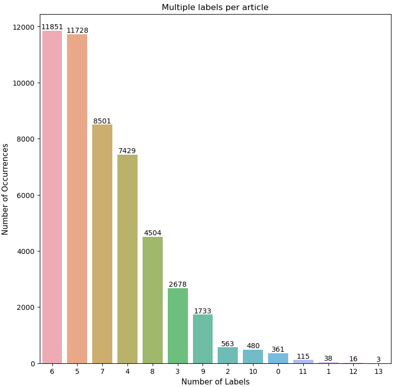
Most of the articles have 6 or 5 labels.

Dataset cleaning

We saw that there are 361 documents without any label so they are considered as a noise for the model because they don’t have any valuable information. Before doing any text preprocessing we will eliminate these rows.

check_row =[]
for sum in rowsums.values:
    check_row.append(sum)
trimmed_dataframe['check'] = check_row 
trimmed_dataframe = trimmed_dataframe.drop(trimmed_dataframe[trimmed_dataframe['check']==0].index)  

Data preprocessing

This step involves the use of natural language processing techniques and is extremely important before training any ML model because it allows cleaning the data and removing any unnecessary text.

We must design a pre-processing pipeline which will gradually clean the unstructured text at each step. To do this, we will use an already trained pipeline from spaCy library accessible through the method pipe. This method allows pre-processing texts as stream and buffers them in batches, which is much more efficient and quicker. The pre-processing steps applied to our text are the following:

tokenization
lemmatization
lowercasing of all the words
removing of accents, if any
removing of non-alpha words
removing of stop words
removing of digits

import spacy
from tqdm import tqdm
from unidecode import unidecode
spacy.cli.download("en_core_web_sm")

def preprocess_text(lines):
    NLP = spacy.load("en_core_web_sm")  
    final_text = []
    for doc in tqdm(NLP.pipe(lines, batch_size=500), total=len(lines)):
        words = [unidecode(t.lemma_.lower()) for t in doc
                 if t.is_alpha and not t.is_stop and not t.is_digit]
        final_text.append(" ".join([x for x in words if x]))
    return final_text
    
trimmed_dataframe['abstractText'] = preprocess_text(trimmed_dataframe['abstractText'])

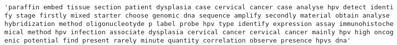
Here is a sample of the original text, before applying the pre-processing pipeline:

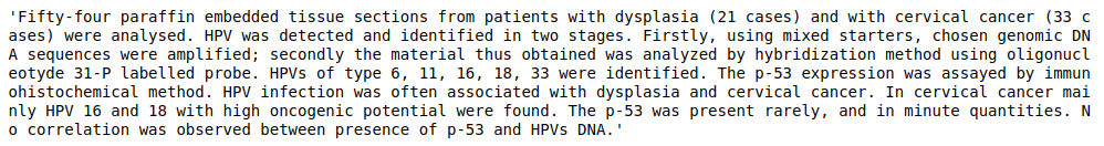
After applying the pre-processing pipeline to our text, the same sample of text looks like this:

Training

Split dataset

First, let’s split the dataset into 2 distinct sets, one for training and one for test. The test dataset represents 20% of the dataset with at least one label, so 9928 documents. Therefore, the model will be trained on 39711 documents.

from sklearn.model_selection import train_test_split

trimmed_dataframe['tokens'] = trimmed_dataframe['abstractText'].apply(lambda x: x.split(" "))
X = trimmed_dataframe['tokens']
y = np.asarray(trimmed_dataframe[trimmed_dataframe.columns[1:15]])

X_train, X_test, y_train, y_test = train_test_split(X, y, test_size=0.2)

Convert data into numerical vectors

Because no algorithm understands our human language, we need to convert it into a numerical format, which is called embeddings.

There exist multiple techniques to generate word embeddings and some examples are:

For this blog post, to create word embeddings we use Word2Vec model from gensim library. This model is chosen because it has the capability to learn word relationships and considers the semantic aspects of the text data.

import gensim
from gensim.models import Word2Vec

embedd_model = Word2Vec(sentences = X_train, vector_size=100, window=5, min_count=1)
word_vectors = embedd_model.wv

To generalize the embeddings and to limit the size of an embedded document we will calculate the sentence embedding as an average of the embeddings of each word contained in the sentence.

def sent_vec(sent):
    wv_res = np.zeros(word_vectors.vector_size)
    ctr = 1
    for w in sent:
        if w in word_vectors:
            ctr += 1
            wv_res += word_vectors[w]
    wv_res = wv_res/ctr
    return wv_res
   
X_train_vec = X_train.apply(sent_vec)
X_test_vec = X_test.apply(sent_vec)

Model training and testing

The model that we will train with our training data is Logistic Regression, a linear model from sklearn library. By default, logistic regression models a binary outcome, so it would work with a dataset which has only two labels like yes/no, for example.

This is not such a big problem because we can wrap our logistic regression model with a MultiOutputClassifier object. The strategy behind this object is to train one classifier per label, so for this dataset, 14 classifiers will be trained internally and each classifier will be able to predict if a specific text falls into its category or not.

from sklearn.multioutput import MultiOutputClassifier
from sklearn.linear_model import LogisticRegression

clf = MultiOutputClassifier(LogisticRegression(max_iter=5000)).fit(X_train_vec.to_list(), y_train)

After training the model, we will use it to predict the labels for the 9928 documents from the test set.

from sklearn import metrics
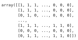
predicted = clf.predict(X_test_vec.to_list())

The prediction result is an array of labels for each MeSH category, where each row represents a document and each column represents a label.

To evaluate a multi-label classifier we have to average the scores obtained by each class. To do this, we will use the micro-averaging and we will calculate the evaluation metrics: precision, recall and the f1 score.

from sklearn import metrics

print('Precision Score: ', metrics.precision_score(y_test, predicted, average="micro"))
print('Recall Score: ', metrics.recall_score(y_test, predicted, average='micro'))
print('F1 Score: ', metrics.f1_score(y_test, predicted, average='micro'))

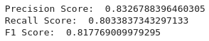
We can see that following a simple method of classification we achieved a precision of 0.83 which means that in 83% of the time the model is correct when predicting the target class. Moreover, the recall is 0.80 which means that in 80% of the time the model finds all objects of the target class. F1 score is calculated as a harmonic mean and is based entirely on precision and recall.

The dataset is imbalanced, as reminded earlier, so it is interesting to see the performance for each label. We can achieve these results by calculating the classification report.

print(metrics.classification_report(y_test, predicted, target_names = trimmed_dataframe.columns[1:15] ))

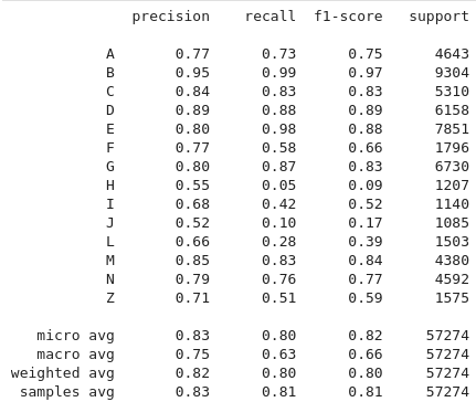
As expected, the classes with a smaller number of documents have a lower performance. The class B with almost 10000 documents is the most performant.

Conclusion

In this article we presented a simple method for building an algorithm for multi-label text classification, but this method is not unique. There are several models that could deal with multi-label classification, like LinearSVC, Neural Network models or pre-trained models like BERT. When we are facing a classification or any other ML task, it is recommended to test multiple algorithms and to choose the one that best suits the requirements of our problem.

We also notices that the data used is highly imbalanced so a first improvement would be trying to balance the dataset by using techniques like SMOTE. We can further improve our model by detecting over-fitting using cross-validation techniques, by doing threshold optimization using ROC Curve or by doing hyperparameter tuning. Because hyperparameter tuning can sometimes be very time-consuming, OPTUNA provides a framework for automatizing the hyperparameter optimization.