31 Jan 2024

Gilles Habran
IT Architect

Data pipelines with Databricks Delta Live Tables

In the world of big data and analytics, being able to efficiently process a large amount of data and drive informed decision-making is a great advantage for data driven companies.

Databricks provides a unified analytics platform that seamlessly integrates with popular data science and machine learning libraries. The platform simplifies the complexities of big data processing, allowing data engineers, data scientists, and data analysts to collaborate and gain knowledge from massive datasets. If you are familiar with Spark (Python, Scala, …), Jupyter notebooks, and SQL; you will most likely enjoy using this platform.

At the heart of the Databricks ecosystem lies Delta Lake, a powerful storage layer that brings reliability and performance to data lakes. Delta Lake introduces ACID transactions, schema enforcement, and scalable metadata management, addressing some of the longstanding challenges associated with big data processing. Delta Lake, initially created by Databricks, is now a Linux Foundation project and thus uses an open governance model.

The Databricks platform is deployed in your cloud environment (AWS, Azure, GCP) close to your data. You are billed for the cloud resources that Databricks use and some Databricks units per hour (DBU/h).

With the importance of real-time data processing, Databricks introduces Delta Live Pipelines which enables us to build end-to-end data workflows from a simple notebook.

From Databricks DLT product description: “Delta Live Tables (DLT) is a declarative ETL framework for the Databricks Data Intelligence Platform that helps data teams simplify streaming and batch ETL cost-effectively. Simply define the transformations to perform on your data and let DLT pipelines automatically manage task orchestration, cluster management, monitoring, data quality and error handling.”

In this post, we create a Delta Live Pipeline using the dlt Python library to process a small dataset about movie ratings. As recommended by Databricks, we follow the Medallion architecture to organize our data:

Bronze zone: raw data ingested in the platform
Silver zone: cleaned data
Gold zone: curated data used by reporting tools and business users

At the end of the processing pipeline, we create a reporting dashboard that displays the data from the Gold zone.

Dataset

The data we use is the Netflix TV shows and movies dataset which contains information such as title, description, release data, ratings, etc…

More information about the dataset and the download link can be found on Kaggle.

Setup

Before working with the data, it is imperative to establish the required resources to support the dataset, including cluster creation and data catalog setup.

Clusters

Databricks offers several clusters concepts:

All-Purpose: a single or multi node cluster to execute notebooks.
Job: cluster automatically started and stopped after a Spark job or when a pipeline has finished.
SQL Warehouse: a Databricks feature for executing SQL queries on platform data through a UI.

For this experiment, we have configured both a single-node cluster and a SQL Warehouse. The single node cluster allows us to run notebook, while the SQL Warehouse Cluster gives us the possibility to run SQL queries to explore our data catalog.

The single node cluster has the following configuration:

Databricks runtime version 13.3 LTS (Spark 3.4.1)
8GB memory
2 cores

The SQL Warehouse cluster is configured as follows:

Name: blog-sql-warehouse
Cluster size: 2X-Small
Scaling: Min 1, Max 2
Type: Pro

Setup the data catalog

Once our cluster is operational, we can attach notebooks and configure our environment with SQL commands or a scripting language like Python. Specifically, for our experimentation, we need to create a database and a volume. A volume, in Databricks terms, represents a logical volume of storage in the cloud.

To achieve this:

connect to the Databricks console,
Create a notebook called blog-dlt-setup, and connect it to our cluster,
Open the notebook,
Copy/Paste the following instructions in the notebook’s cell, and execute it:

%sql  # Magic command to inform the cluster that the cell contains SQL commands.
use catalog main;  # Specify to use the catalog 'main'

create database blog;
create volume main.blog.data;  # Create a volume in 'main/blog/data/'

With these steps, the database is set up in our main catalog, and we can now upload our dataset to our volume using the Databricks console.

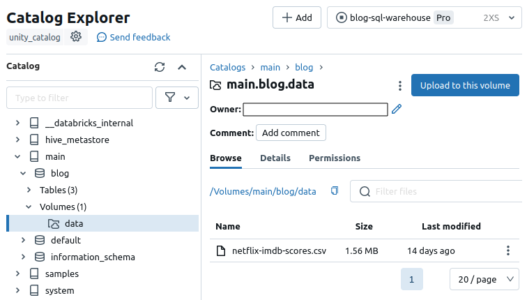
Once uploaded, the dataset becomes available to our notebooks with the path /Volumes/main/blog/data/netflix-imdb-scores.csv

Quick overview of the data

In this section, we conduct a brief examination of the data previously uploaded to discern our objectives for the upcoming pipeline.

To initiate this process, we create a notebook named blog-dlt-pipelines-eda in our workspace and attach it to our running cluster.

As a disclaimer, it is important to acknowledge that the primary aim is to showcase a Databricks Delta Live pipeline in action. Consequently, some data transformation and cleaning procedures may deviate from the best practices of data preparation, as they are not the focal point of this post.

Let’s first start by creating a PySpark dataframe with our dataset.

from pyspark.sql.functions import *

dataset_path = "/Volumes/main/blog/data/netflix-imdb-scores.csv"
df = spark.read.options(delimiter=",", header=True, multiline=True).csv(dataset_path)

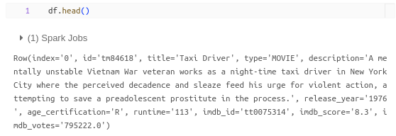
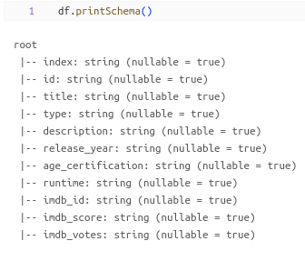
Then, we can check the first rows and the schema of our data.

df.head()

df.printSchema()

For the purposes of this post, let’s assume our objective is to visualize the number of movies and shows released each year, along with the average ratings per year. To achieve this, we need to preprocess the data for usability, and one effective approach is to create a Delta Live Pipeline.

Delta Live Pipeline

We create a Delta Live Pipeline by defining one in a notebook and subsequently executing it in a workflow.

Notebook

Firstly, we create a new notebook titled blog-dlt-pipelines where the Delta Live Pipeline is crafted.

This notebook encapsulates the transformations intended for execution, outlined as follows:

Creation of a Bronze table containing raw data;
Formation of a Silver table comprising cleaned data;
Generation of a Gold table containing data tailored for our dashboard.

The code to be executed is presented below, with comments providing context:

import dlt
from pyspark.sql.functions import *
from pyspark.sql.types import *

dataset_path = "/Volumes/main/blog/data/netflix-imdb-scores.csv"  # Path to the dataset on the volume


@dlt.table(
    comment="Raw data - Netflix IMDB scores from Kaggle: https://www.kaggle.com/datasets/thedevastator/netflix-imdb-scores/",
    name="main.blog.bronze_netflix_imdb_scores",
    temporary=False
)
def netflix_imdb_raw():  # Function that read the CSV file from the Volume, and create a table called bronze_netflix_imdb_scores
    return (spark.read.options(delimiter=",", header=True).csv(dataset_path))

columns_to_drop = ["index", "id", "title", "description", "age_certification", "imdb_id"]
@dlt.table(
    comment="Silver data - Netflix IMDB scores without irrelevant columns, multiline data not read properly, and numeric data cast as float or int",
    name="main.blog.silver_netflix_imdb_scores",
    temporary=False
)
def netflix_imdb_silver():
    return (
        dlt.read("main.blog.bronze_netflix_imdb_scores")  # Read the bronze table
            .drop(*columns_to_drop)  # Drop unwanted columns
            .withColumn("release_year", col("release_year").cast('int'))  # Cast column to int
            .withColumn("runtime", col("runtime").cast("float"))  # Cast column to float
            .withColumn("imdb_score", col("imdb_score").cast("float"))
            .withColumn("imdb_votes", col("imdb_votes").cast("float"))
            .where( ((col("type") == "SHOW" ) | (col("type") == "MOVIE")) & col("release_year").isNotNull() )  # Keep only rows with type as MOVIE or SHOW and with a non-null release_year
    )

@dlt.table(
    comment="Gold data - Netflix IMDB scores with aggregations",
    name="main.blog.gold_netflix_imdb_scores",
    temporary=False
)
def netflix_imdb_gold():
    return (
        dlt.read("main.blog.silver_netflix_imdb_scores")  # Read the silver table
            .groupBy("release_year", "type")  # Group by release year and type
            .agg(count("*").alias("release_count"), avg("imdb_score").alias("avg_imdb_score"), avg("imdb_votes").alias("avg_imdb_votes"))  # Aggregate columns of interest
    )

This notebook can now be used in a workflow to create and execute the pipeline.

Workflow

The configuration of the DLT pipeline is managed in the Workflows -> Delta Live Tables menu of Databricks console.

We give it the following properties:

Pipeline name: blog-dlt-pipeline
Pipeline mode: Triggered as we want a one time run
Paths: the path to our pipeline notebook
Storage options: Unity Catalog
Catalog: main
Target schema: blog
Cluster mode: Fixed Size
Workers: 1
Instance profile: None

Finally, clicking on create and start initiates the workflow. Upon successful execution, the workflow status can be observed, as depicted in the following image:

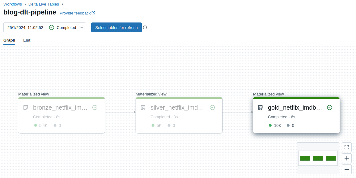
Results

After the successful execution of the Delta Live Pipeline, we can validate the applied transformations by examining our tables using either the SQL Warehouses feature or directly from a notebook.

In our case, we leverage the SQL warehouse cluster established at the beginning of the configuration.

To perform the inspection, access the SQL Editor menu in the Databricks console and select the cluster named blog-sql-warehouse.

We first check the bronze table with following query:

select * from main.blog.bronze_netflix_imdb_scores limit 1;

Then the silver table:

select * from main.blog.silver_netflix_imdb_scores limit 1;

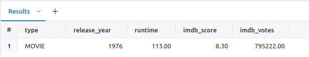
And finally, the gold table:

select * from main.blog.gold_netflix_imdb_scores limit 1;

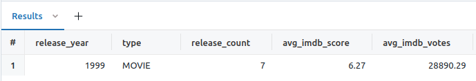
All three tables exhibit the expected output.

Dashboard

A dashboard is a collection of diagrams based on saved SQL queries. Our dashboard uses the two queries below.

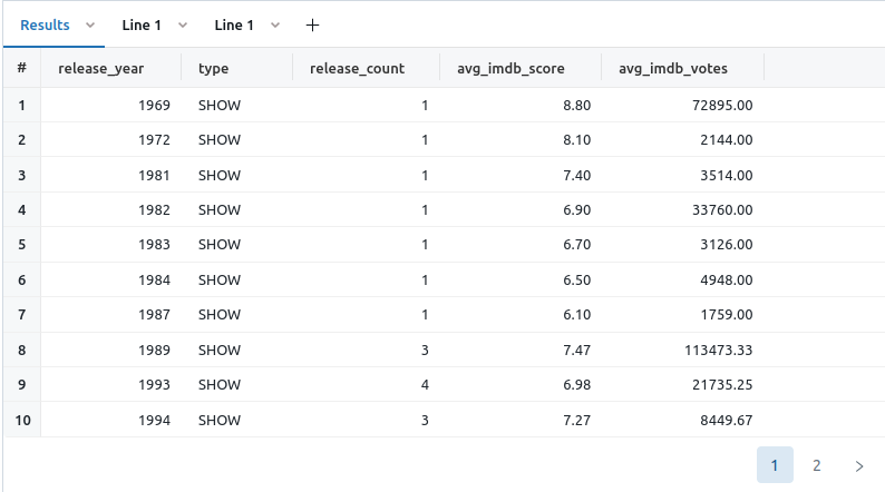
Query 1: gold_shows

select * from main.blog.gold_netflix_imdb_scores where type = "SHOW" and release_year < (select MAX(release_year) from main.blog.gold_netflix_imdb_scores) order by release_year;

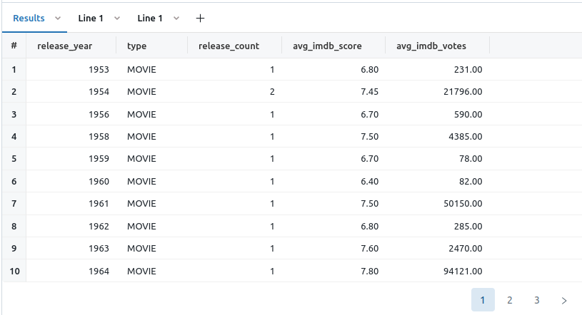
Query 2: gold_movies

select * from main.blog.gold_netflix_imdb_scores where type = "MOVIE" and release_year < (select MAX(release_year) from main.blog.gold_netflix_imdb_scores) order by release_year;

With these queries saved, we proceed to construct our dashboard in the Dashboards menu of the Databricks console.

When creating a visualization widget, the data source is specified as the saved SQL query. Once configured, we can define the visualization type, columns for X/Y, and additional configurations such as scaling, colors, and data labels.

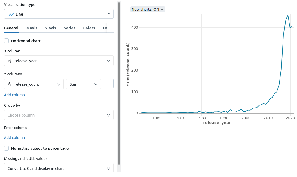
After adding a few widgets, the end result is a dashboard that can be refreshed manually or scheduled:

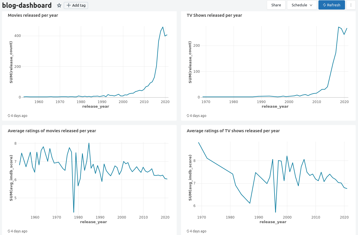
Conclusion

Our exploration of Databricks Delta Live Tables demonstrated seamless data pipeline creation and validation. Leveraging Delta Lake’s features and Databricks’ collaborative environment, we efficiently processed a Netflix dataset through Medallion architecture.

The setup involved configuring clusters and the data catalog, while Delta Live Pipelines effortlessly organized data into Bronze, Silver, and Gold tables. Results validation confirmed expected outcomes in these tables.

This journey showcased the efficiency of Databricks Delta Live Tables, from raw data processing to curated datasets and interactive dashboards, making it a valuable tool in the dynamic realm of big data and analytics. Additionally, as our data grows, the platform allows for easy configuration of auto-scaling in our processing clusters to handle increased demands.